CVPR 2019에서 발표된 MRI Reconstruction 관련 논문으로, 1) MRI reconstruction 과정에서 uncertainty를 함께 측정하였으며, 2) 별도의 evaluator network를 이용하여 매 시점에서 다음 sampling할 위치를 찾는 active sampling을 수행했다.
Introduction
🍏 Uncertainty에는 model uncertainty와 data uncertainty 두 가지가 있다. Model uncertainty는 모델이 완벽하지 않을 때 발생하는 예측값의 불확실성이고, data uncertainty는 데이터 자체에 내재된 불확실성이다. MRI reconstruction의 경우에는 k-space에서 데이터의 일부만 얻은 후 나머지 부분을 복원하는 것을 목적으로 하기 때문에, 여기에서 data uncertainty가 기인한다고 볼 수 있다.
🍏 본 논문에서는 MRI reconstruction에서 발생하는 data uncertainty를 측정한다. 여기서 측정한 data uncertainty를 줄이는 방향으로 다음 sampling할 위치를 하나씩 찾는 active sampling을 도입하여 효과적으로 MRI를 복원할 수 있다.
Background and notation
본 논문에서 사용하는 notation은 다음과 같다.
- y∈CN×N: full-sampled k-space data
- x=F−1(y)∈CN×N: full-sampled image
- $\text{S}: binary sampling mask (k-space Cartesian acquisition trajectory)
- ˆy=S⊙y: undersampled k-space data
- ˆx=F−1(ˆy): undersampled image (zero-filled reconstruction)
🔅 또한, 본 논문에서는 complex MRI data를 이용하지 않고 magnitude 값만을 이용했다. 즉, k-space 데이터는 다음과 같이 얻어진다.
- y=F(abs(x))
Method

본 논문에서 제안한 framework는 두 가지의 네트워크로 구성되어 있다.
(1) Reconstruction network: undersampled image를 복원하고 uncertainty map을 추정한다.
(2) Evaluator: 복원된 이미지의 각 k-space row의 점수를 평가한다.
Reconstruction network는 encoder-decoder residual network + DC layer이 3번 반복되는 구조로 되어 있다.
🎈 DC layer은 다음과 같이 표현될 수 있다.
- r=DC(ˆx,S)=F−1((1−S)⊙F(f(ˆx))+S⊙F(ˆx))
즉, observed row에 대해서는 해당 값(F(ˆx))을 사용하고, unobserved row에 대해서는 Reconstruction network로 복원된 값(F(f(ˆx)))을 사용한다. 이는 CascadeNet에서 제안된 DC layer의 noiseless version이다.
🎈 Reconstruction network는 undersampled image를 복원하는 것 외에도 pixel-wise uncertainty map u(ˆx)을 함께 추정한다. 이를 위해 average conditional log-likelihood를 최대화하는 loss를 이용한다.
- LR(ˆx,r,x)=1N2∑N2i=1|ri−xi|22u(ˆx)i+12log(2πu(ˆx)i)
큰 uncertainty 값을 갖는 부분은 큰 reconstruction error을 가질 확률이 높음을 의미한다. 이렇게 계산된 uncertainty map은 active acquisition을 멈추는 기준(halting signal)으로 이용된다.
- Reconstruction network
#https://github.com/facebookresearch/active-mri-acquisition/blob/2780bd93d0849ba060a60ee264d7dd407bd68162/activemri/experimental/cvpr19_models/models/reconstruction.py#L112

class ReconstructorNetwork(nn.Module):
    def __init__():
        ...

        decoder = []
        ... # decoder layers
        decoder.append(nn.Conv2d(num_filters, 3, 1)) #out_channel=3 (real+imag+uncertainty map)
        self.decoders = nn.Sequential(*decoder)

        ...


    def forward():

        for i, (encoder, residual_bottleneck, decoder) in enumerate(
            zip(self.encoders, self.residual_bottlenecks, self.decoders)
        ):
            encoder_output = encoder(encoder_input)

            #residual connection
            if i > 0:
                encoder_output = encoder_output + residual_bottleneck_output

            residual_bottleneck_output = residual_bottleneck(encoder_output)

            decoder_output = decoder(residual_bottleneck_output)

        	#output
            recon_image = self.data_consistency(decoder_output[:, :-1, ...], zero_filled_input, mask)
            uncertainty_map = decoder_output[:, -1:, ...]

        ...

return reconstructed_image, uncertainty_map- Loss
#https://github.com/facebookresearch/active-mri-acquisition/blob/main/activemri/experimental/cvpr19_models/models/fft_utils.py#L92

import torch.nn.functional as F

def gaussian_nll_loss(reconstruction, target, logvar, options):
	reconstruction = to_magnitude(reconstruction)
	target = to_magnitude(target)
	l2 = F.mse_loss(reconstruction, target, reduce=False)
	#Clip logvar to make variance in [0.0001, 5], for numerical stability
	logvar = logvar.clamp(-9.2, 1.609)
	one_over_var = torch.exp(-logvar)

	return 0.5 * (one_over_var * l2 + logvar)
Evaluator network의 목적은 k-space의 각 row가 진짜인지, 복원된 값인지 평가하는 것이다. 이는 adversarial learning과 유사한데, 이를 통해 작은 구조적 차이까지도 포착하여 실제 distribution과 매우 유사한 이미지를 복원할 수 있다.
🎈 Evaluator network e(r,S)의 작동 순서는 다음과 같다.
- Reconstructed image r∈CN×N을 N개의 spectral map으로 분해한다. 이 때 각 spectral map은 하나의 k-space row에 해당한다.

- M(r)(i)=F−1(ˆS(i)⊙F(r))
- 즉, k-space에서 하나의 (i-th) line만을 이용해 FT를 한 이미지를 의미한다.
- 비슷하게, GT image를 N개의 spectral map으로 분해한다. →M(x)(i)
- acquisition trajectory S를 6D vector로 embedding한다 (코드에서는 이 부분을 Reconstruction network에 구현했다)
- Spectral map과 trajectory embedding을 CNN에 input으로 넣는다.
- Observed row에 해당하는 spectral map에는 높은 값을, unobserved row에 해당하는 spectral map에는 낮은 값을 예측하게 하도록 evaluator을 학습시킨다.
- 이때, 가장 간단한 방법은 binary classifier을 학습시켜 0과 1로 구분하도록 하는 것인데, 이 경우 잘 학습이 되지 않았다고 한다.
- 이 대신, GT spectral map을 함께 이용하는 target score function t(r,x)을 정의한 후, 이 target score을 예측하게 하는 방식으로 학습을 진행한다.
- t(r,x)i=exp(−γ||M(r)(i)−M(x)(i)||22)
- M(r)(i)이 M(x)(i)과 유사할수록, target score은 1에 가까워진다.
- Evaluator의 loss는 다음과 같게 된다.
- LEE(r,x,S)=∑Ni|e(r,S)i−t(r,x)i|2
- Reconstruction network에서 mask embedding을 함께 예측한다.
class ReconstructorNetwork(nn.Module):
    def __init__(self, mask_embed_dim=6):
        self.mask_embedding_layer = nn.Conv2d(img_width, mask_embed_dim, 1, 1)
        ...

    def embed_mask(self, mask):
        b, c, h, w = mask.shape
        mask = mask.view(b, w, 1, 1)
        return self.mask_embedding_layer(mask) #b, mask_embed_dim, 1, 1

    def forward(self, zero_filled_input, mask):
        mask_embedding = self.embed_mask(mask).repeat(1,1,*zero_filled_input.shape[2:])
        encoder_input = torch.cat([zero_filled_input, mask_embedding], 1)
        ...
return reconstructed_image, uncertainty_map, mask_embedding- Evaluator network는 Reconstruction network에서 계산한 reconstructed image, mask embedding, mask를 input으로 받는다.
class EvaluatorNetwork(nn.Module):
    def __init__(self, ):
        self.spectral_map = SpectralMapDecomposition()
        self.model = #2dcnn

    def forward(self, input_tensor, mask_embedding, mask):
        spectral_map_and_mask_embedding = self.spectral_map(input_tensor, mask_embedding, mask)
        out = self.model(spectral_map_and_mask_embedding)
return out- Spectral Map Decomposition
class SpectralMapDecomposition(nn.Module):
    def __init__(self):
        super().__init__()

    def forward(self, reconstructed_image, mask_embedding, mask):
        b, _, h, w = reconstructed_image.shape

        kspace = fft(reconstructed_image).unsqueeze(1).repeat(1, w, 1, 1, 1) #b, w, c, h, w

        separate_mask = torch.zeros([1, w, 1, 1, w])
        for i in range(width):
            separate_mask[0, i, 0, 0, i] = 1

        masked_kspace = torch.where(separate_mask.byte(), kspace, torch.tensor(0.0))
        masked_kspace = masked_kspace.view(b*w, 2, h, w)

        separate_images = ifft(masked_kspace)
        separate_images = separate_images.view(b, 2, w, h, w)

        #add mask information as a summation
        separate_images = separate_images + mask.permute(0,3,1,2).unsqueeze(1).detach()
        separate_images = separate_images.view(b, 2*w, h, w)

        spectral_map = torch.cat([separate_images, mask_embedding], dim=1)
        return spectral_map
🎈 Evaluator network는 또한 reconstruction network의 업데이트에 함께 이용된다. 이를 통해 reconstruction network는 높은 evaluator score을 얻는 방향으로 학습하게 된다.
- LRE(r,S)=∑Ni|e(r,S)i−1|2
Reconstruction network의 최종 loss는 다음과 같게 된다.
- L(R,x,S)=1K∑Kk=1LkR(rk−1,rk,x)+βLRE(rK,S)
reconstructor.train()
zero_filled_image, target, mask = batch

reconstructed_image, uncertainty_map, mask_embedding = reconstructor(zero_filled_image, mask)

#update evaluator
evaluator.train()
optim_D.zero_grad()

fake = reconstructed_image.detach()
mask_embedding = mask_embedding.detach()
output = evaluator(fake, mask_embedding, mask)
loss_D_fake = loss_GAN(output, False, mask, fake, target)

real = target
output = evaluator(real, mask_embedding, mask)
loss_D_real = loss_GAN(output, True, mask, fake, target)

loss_D = loss_D_fake + loss_D_real
loss_D.backward()
optim_D.step()

output = evaluator(reconstructed_image, mask_embedding, mask)
loss_G_GAN = loss_GAN(output, True, mask, reconstruted_image, target)

#update reconstructor
optim_G.zero_grad()
loss_G = loss_NLL(reconstructed_image, target, uncertainty_map).mean()
loss_G += loss_G_GAN
loss_G.backward()
optim_G.step()
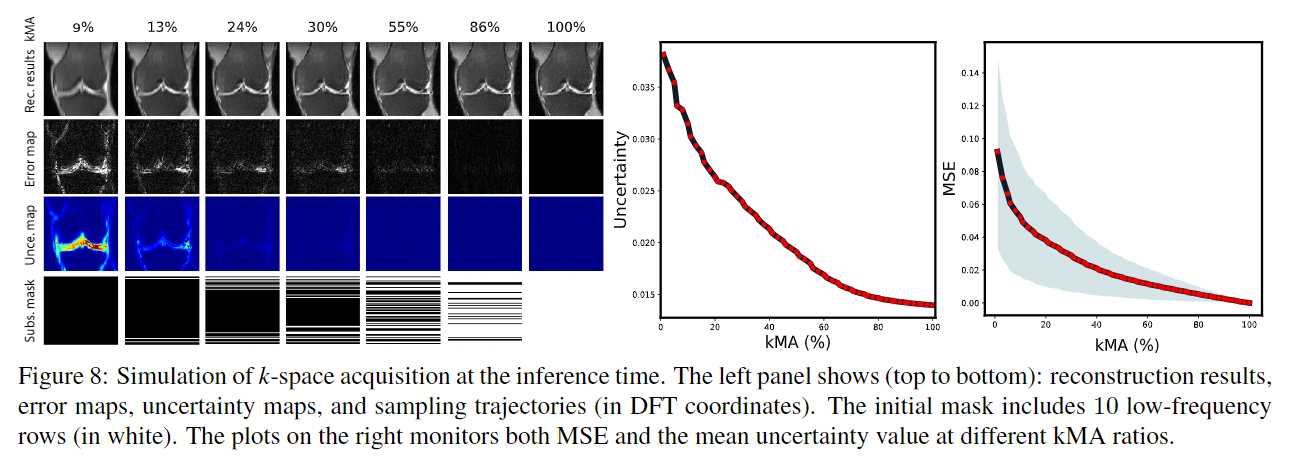
🎈 Inference time에는, evaluator score은 다음으로 얻을 k-space line의 위치를 결정하는 데에 이용된다. Acquire -> reconstruction의 과정을 stopping criteria를 만날 때까지 반복한다.
Experiments
💡 fastMRI knee dataset의 일부를 실험에 사용했다. 11,049개의 train data와, 5,048개의 validation data를 사용했다.
💡 전체 k-space line 수에 대해 얻은 k-space line의 수의 비율을 kMA로 표기했다. (kMA = (# of acquired measurements) / (# of all possible measurements))
💡 처음 sampling trajectory로는 low frequency에서 10개의 line을 이용했고 (7.8% kMA), 한 줄씩 추가로 얻어가는 과정을 반복했다.