CVPR 2021에 발표된 MR reconstruction 관련 논문이다. Model-based method를 이용하여 k-space와 image domain 둘 다에서 reconstruction을 진행하고, coil sensitivity map 역시 CNN으로 계산하여 fastMRI 2020 challenge에서 2위를 차지했다.
Introduction
Deep learning을 이용한 MR reconstruction은 크게 두 가지로 분류할 수 있다.
1) Direct mapping: image domain 혹은 k-space에서 바로 target image를 reconstruction하거나, manifold learning을 이용해 missing k-space data를 estimation 하는 방법.
2) Model-based methods: coil sensitivity map, k-space sampling matrix 등의 사전정보를 활용하여, deep learning algorithm을 regularization function으로써 사용하는 unrolled architecture을 이용하는 방법. MoDL (Model Based Deep Learning Architecture for Inverse Problems), KIKI-net, Deep CascadeNet 등이 여기에 속한다.
Problem Formulation
multi-coil MR image acquisition은 다음과 같이 정의할 수 있다.
$Ax + n = b$ ... (1)
- $x \in \mathbb{C}^N$ : desired MR image
- $b \in \mathbb{C}^{NN_c}$ : measured multi-coil k-space
- $A:\mathbb{C}^N\rightarrow\mathbb{C}^{NN_c}$ : coil sensitivity map $C$, Fourier transform $\mathcal{F}$, k-space sampling matrix $M$ 등을 포함하는 forward model
일반적으로, MR reconstruction에서 풀고자 하는 문제는 다음과 같다.
$\min_x||Ax-b||^2_2+\lambda$$\mathcal{R}(x)$ ... (2)
그러나 본 논문에서는 여기에 coil sensitivity map estimation까지 추가해서 최종적으로 다음과 같이 문제를 정의한다.
$\min_{x, C}||Ax-b||^2_2+\lambda_x$$\mathcal{R}(x)$$+\lambda_C$$\mathcal{R}(C)$ ... (3)
Coil sensitivity map estimation이 필요한 이유는 다음과 같다.
1) Calibration scan data를 이용해 pre-acquire하는 경우: scan time이 증가하고, 실제 subject image와 inconsistent할 수 있음.
2) ACS line을 이용해 pre-compute하는 경우: acceleration factor가 높을 경우 부정확할 수 있음.
Joint Reconstruction of Image and Coil Sensitivity Map
Eq. (3)의 image $x$에 대한 regularization term (두 번째 항)을 다음과 같이 정의한다.
- $\mathcal{R}(x)$$=||x-\mathcal{D}_I(x)||^2_2 + ||x-\mathcal{F}^{-1}\mathcal{D}_F(f)||^2_2$ ... (4)
- $f=\mathcal{F}(x)$ : k-space of $x$
- $\mathcal{D}_I$ : $x$로부터 reconstruction을 진행하는 de-aliasing model
- $\mathcal{D}_F$ : $f$로부터 missing k-space data point에 대한 interpolation을 진행하는 k-space model
설명하는 바는 다르지만 결국 $\mathcal{D}_I$와 $\mathcal{D}_F$ 둘 다 reconstruction을 하는 network이고, 전자는 image domain에서의 reconstruction을 수행하며 후자는 k-space에서의 reconstruction을 수행한다는 점만 다르다.
Eq. (3)의 coil sensitivity map $C$에 대한 regularization term (세 번째 항)을 다음과 같이 정의한다.
- $\mathcal{R}(C)$$=||C-\mathcal{D}_C(\mathcal{F}^{-1}b)||^2_2$ ... (5)
- $\mathcal{D}_C$ : acquired k-space data $b$로부터 coil sensitivity map을 estimation하는 coil sensitivity model
두 regularization term을 Eq. (3)에 대입하면 다음과 같다.
- $\min_{x, C}||Ax-b||^2_2+\lambda_I||x-\mathcal{D}_I(x)||^2_2 + \lambda_F||x-\mathcal{F}^{-1}\mathcal{D}_F(f)||^2_2 + \lambda_C||C-\mathcal{D}_C(\mathcal{F}^{-1}b)||^2_2$ ... (6)
위 식을 두 variable $x$, $C$에 대해 각각 분리하면 다음과 같다.
- $\min_{x}||Ax-b||^2_2+\lambda_I||x-\mathcal{D}_I(x)||^2_2 + \lambda_F||x-\mathcal{F}^{-1}\mathcal{D}_F(f)||^2_2$ ... (7)
- $\min_{C}||Ax-b||^2_2 + \lambda_C||C-\mathcal{D}_C(\mathcal{F}^{-1}b)||^2_2$ ... (8)
두 equation을 gradient descent method를 이용하면 iterative하게 풀어낼 수 있다. 이때 $\mu_k$, $\nu_k$는 step size이다.
- $x_{k+1}=x_k-2\mu_k[A^*(Ax_k-b)+\lambda_k^I(x_k-\mathcal{D}_I(x_k))+\lambda_k^F(x_k-\mathcal{F}^{-1}\mathcal{D}_F(f))]$ ... (9)
- $C_{k+1}=C_k-2\nu_k[\mathcal{F}^{-1}M^T(Ax_k-b)x_k^*+\lambda_k^C(C_k-\mathcal{d}_C(\mathcal{F}^{-1}b))]$ ... (10)
Methods


Joint IC-Net은 위 두 equation을 이용해 설계되었으며, 두 개의 main block으로 이루어져 있다.
1) MR image reconstruction block: MR image를 image domain과 k-space에서 각각 reconstruction 하고, MR image에 대한 data consistency layer을 포함한다.
2) Coil sensitivity maps reconstruction block: Coil sensitivity map을 estimation하고, coil sensitivity map에 대한 data consistency layer을 포함한다.
MR image reconstruction block.
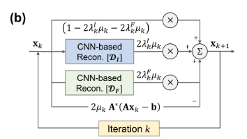
Eq. (9)는 다음과 같이 정리할 수 있다.
$x_{k+1}=(1-2\lambda_k^I\mu_k-2\lambda_k^F\mu_k)x_k$
$+2\lambda_k^I\mu_k\mathcal{D}_I(x_k)$
$+2\lambda_k^F\mu_k\mathcal{F}^{-1}\mathcal{D}_F(f))$
$-2\mu_kA^*(Ax_k-b)$
이 때,
- $\lambda_k^I$, $\lambda_k^F$, $\mu_k$ : trainable parameters
- $\mathcal{D}_I$, $\mathcal{D}_F$ : based on U-net architecture + residual learning
- $\mathcal{D}_F$를 k-space에 대해 train하기 위해, input과 output에 대해 각각 FT와 IFT를 수행한다.
Coil sensivitiy maps reconstruction block.
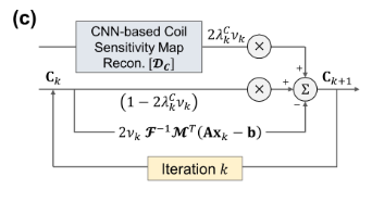
Eq. (10)은 다음과 같이 정리할 수 있다.
$C_{k+1}=(1-2\lambda_k^C\nu_k)C_k$
$+2\lambda_k^C\nu_k\mathcal{D}_C(\mathcal{F}^{-1}b)$
$-2\nu_k\mathcal{F}^{-1}M^T(Ax_k-b)x_k^*$
이 때,
- $\lambda_k^C$, $\nu_k$ : trainable parameters
- $\mathcal{D}_C$ : based on U-net architecture
- $\mathcal{D}_C$는, 이전 network의 reconstruction 결과를 input으로 사용하는 $\mathcal{D}_I$, $\mathcal{D}_F$와 다르게 항상 undersampled k-space를 input으로 사용한다. 전체 architecture (a)를 참고.
Unfolded Network
학습은 end-to-end로 진행되고, SSIM loss를 사용한다.
$\mathcal{L}=\sum_{N_S}(1-\text{SSIM}(|x_{N_k}|, |x_T|))$
Implementation
- MR image의 경우, complex data이기 때문에 real-value로 만들기 위해 real part와 imaginary part를 각각 channel 별로 concatenate했다.
- Model:
- Unet with 4 layers in each encoder and decoder part
- Each conv block consists of {2D conv, leaky ReLU (a=0.2), InstanceNorm}
- feature map size starts from 32, 32, 4 for $\mathcal{D}_I$, $\mathcal{D}_F$, $\mathcal{D}_C$, doubled after each max-pooling layer and halved after each up-sampling layer
- $\lambda_k$, $\mu_k$, $\nu_k$ : initialized as 1
- total iterations $N_k$ = 10
- Before calculating loss, a root sum-of-squares (RSS) operation was applied to the output and the target.
- Optimizer: Adam with $\beta_1=0.9$ and $\beta_2=0.999$ with lr=0.0005
- Number of epochs = 50
- Total training time : 48 hrs with 8 NVIDIA TITAN RTX (24 GB each)
- Dataset : fastMRI multicoil brain dataset
- Evaluation metrics: NRMSE, PSNR, SSIM
Experiments
- Competitors: l1-ESPIRiT, Unet, k-space learning, DeepCascade
- Ablation studies:
- different $N_k$
- replace $\mathcal{D}_C$ by ESPIRiT
- without k-space regularization $\mathcal{D}_F$
- without DC layers
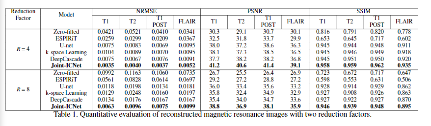
Results
Comparison with other reconstruction methods.
다양한 비교대상과의 실험에서 가장 높은 성능을 보였다.
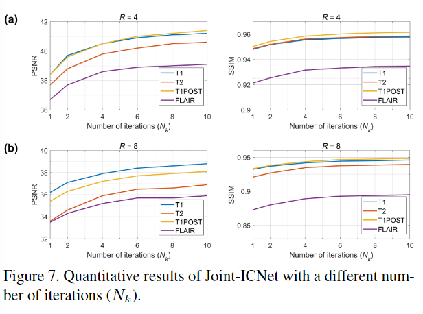
Ablation study of Joint-ICNet
iteration 수가 높아질수록 성능이 높아짐을 보였으며, 다양한 종류의 variation들과 비교했을 때 Joint-ICNet의 성능이 가장 우수했다.

Ablation study의 종류와 그에 대한 분석이 조금 더 다양했으면 하는 아쉬움이 있으나 성능은 확실히 잘 나오는 듯 하다.
공개 코드가 없는 것도 아쉬운데 구현이 어렵지 않아 보이고 Github에 PyTorch로 구현된 코드가 있다. (링크)